SPACAR Light
Example: Visualizing the effective rotation axis of a rigid body in an eigenmode
When a rigid body is rotating, there is an effective axis around which that rotation is taking place. This axis may pass through the rigid body, but it could also be located entirely outside the body.
When analyzing the eigenmodes of a system, some modes may show significant motion of rigid bodies. Other modes may show mostly flexible deformation, with very little motion of rigid bodies.
For the interpretation of the rigid body motion in an eigenmode, it can be helpful to visualize the effective axis of rotation. This can be done in a post-processing step, following a SPACAR Light simulation, using standard MATLAB plotting commands and a custom script: getpoleaxis.m.zip. The script getPoleAxis.m (case-sensitive) needs to be placed in the same folder as the main script for the model (or at least be available on the MATLAB path).
In the main model script, after out = spacarlight(nodes,elements,nprops,eprops,opt);, we'll add the following lines:
out = spacarlight(nodes, elements, nprops, eprops, opt);

fh = out.fighandle; %handle to the Spavisual window
ah = fh.Children(1); %handle to the axis in the Spavisual window
% view(ah,70,30) %set the desired view angle

i_node = 3; %node number to which the rigid body of interest is connected
i_mode = 1; %number of the eigenmode of interest

%get rotation axis
[screwaxis,screwloc] = getPoleAxis(opt.filename,i_node,i_mode);
Here, we first determine a handle to the axis of the Spavisual window. Then, i_node is set to the number of the node that the rigid body of interest is connected to (in this case node 3). Variable i_mode contains the index of the eigenmode of interest (in this case the first mode). The custom function getPoleAxis then determines the effective axis of rotation. Output variable screwaxis contains a vector that lies along this axis, essentially specifying the orientation of the axis. Output variable screwloc contains the x-,y-,z-coordinates of a point on this rotation axis, which is helpful for determining the position of the axis in space. This point is defined as the point on the axis that has the shortest distance to the specified node i_node.
For plotting, the following lines of code can be used:
%mark the node that was provided, using a black dot
plot3(ah,nodes(i_node,1),nodes(i_node,2),nodes(i_node,3), 'k.', 'MarkerSize', 30);

%mark the point on the rotation axis that is *closest to the provided node*
plot3(ah,screwloc(1),screwloc(2),screwloc(3), 'r.', 'MarkerSize', 30);

%plot the rotation axis corresponding with the rigid body motion occuring in
% the eigenmode with number i_mode
ax = [screwloc screwloc+screwaxis screwloc-screwaxis];
plot3(ah,ax(1,:),ax(2,:),ax(3,:),'r')
Here, we're using the standard MATLAB plotting command plot3 to mark the node i_node, to mark the point on the rotation axis, and to plot the rotation axis itself.
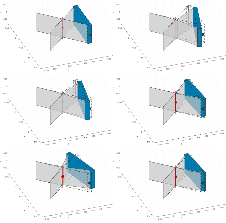
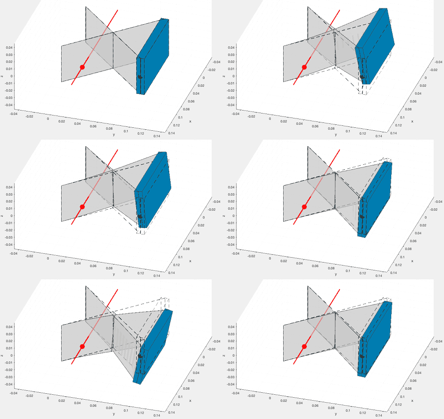
The results for two eigenmodes are shown in the figures below. Node 3 was used, which is one of the nodes connected to the dark blue rigid body stage of the cross-hinge mechanism, and indicated by the black dot.
A few remarks:
- This visualization code is rather crude, in the sense that it's a direct overlay on top of the Spavisual window. We're just computing the coordinates of a line and inserting it into an existing figure. There is no interaction with the Spavisual buttons. So, make sure that the eigenmode you're viewing in Spavisual is the same as the mode that you plotted the rotation axis for.
- If the specified node does not actually rotate in the specified eigenmode, there is no rotation and there will be no effective axis. Calls to
getPoleAxisin that case may not produce an error and probably just lead to incorrect numbers being returned. The same holds in the case that the rigid body is moving as a pure translation: even though there is no effective rotation axis, the script may not produce an error, and just return erroneous numbers, without a warning. - Simulation results in general may be displayed in various load steps (e.g. if a command like
nprops(i).forceornprops(i).displ_xis used, rather thannprops(i).force_initialornprops(i).displ_initial_x). The number of load steps in a simulation result is indicated in the Spavisual window by means of the large horizontal load step slider at the bottom. For each load step, a new set of eigenmodes is shown. ThegetPoleAxisscript, used in this example, uses the eigenmodes that correspond with the first load step. Again, there is no interaction between the Spavisual buttons and this visualization script, so take care to look at the correct eigenmode and the load step. - It is possible that the motion of a rigid body consists of both a rotation about an effective axis and a simultaneous translation along that same axis: the rigid body then makes a screw motion. In this case, the script will return the effective axis.
- rotaxis_example.m
% This example simulates a simple cross flexure
% In the post-processing step, we'll plot the effective rotation axis of
% the rigid body when it moves according to various eigenmodes of the
% system.

clear
clc
% addpath('spacar')		%Specify location of spacar folder, if not current

%% NODE POSITIONS
%           x y z
nodes = [   0 0 0;      %node 1
            0 0.1 0;    %node 2
            0.1 0.1 0;  %node 3
            0.1 0 0];   %node 4


%% ELEMENT CONNECTIVITY
%               p   q
elements = [    1   3;  %element 1
                2   3;  %element 2
                2   4]; %element 3


%% NODE PROPERTIES
%node 1
nprops(1).fix               = true;         %Fix node 1

%node 3
nprops(2).mass              = 0.1;          %Mass [kg] of node 2
nprops(3).mass              = 0.1;          %Mass [kg] of node 3

%node 4
nprops(4).fix               = true;         %Fix node 4


%% ELEMENT PROPERTIES
%Property set 1
eprops(1).elems    = [1 3];            %Add this set of properties to elements 1 and 3
eprops(1).emod     = 210e9;            %E-modulus [Pa]
eprops(1).smod     = 70e9;             %G-modulus [Pa]
eprops(1).dens     = 7800;             %Density [kg/m^3]
eprops(1).cshape   = 'rect';           %Rectangular cross-section
eprops(1).dim      = [50e-3 0.2e-3];   %Width: 50 mm, thickness: 0.2 mm
eprops(1).orien    = [0 0 1];          %Orientation of the cross-section as a vector pointing along "width-direction"
eprops(1).nbeams   = 2;                %Number of beams used to model this element
eprops(1).flex     = 1:6;        	   %Model all six deformation modes as flexible
eprops(1).color    = 'grey';           %Color
eprops(1).opacity  = 0.7;              %Opacity

%Property set 2
eprops(2).elems    = 2;                %Add this set of properties to element 2
eprops(2).dens     = 3000;             %Density [kg/m^3]
eprops(2).cshape   = 'rect';           %Rectangular cross-section
eprops(2).dim      = [50e-3 10e-3];    %Width: 50 mm, thickness: 10 mm
eprops(2).orien    = [0 0 1];          %Orientation of the cross-section as a vector pointing along "width-direction"
eprops(2).nbeams   = 1;                %Single beam for simulating this element is sufficient (since it is rigid)
eprops(2).color    = 'darkblue';       %Color

%% OPTIONAL ARGUMENTS
opt.filename    = 'ex1';     %Filename

%% CALL SPACAR_LIGHT
out = spacarlight(nodes, elements, nprops, eprops, opt);

%%%%%%%%%%%%%
%%% plotting the effective rotation axis of a rigid body, connected to node
%%% i_node, when it moves according to eigenmode with number i_mode.
%%%%%%%%%%%%

fh = out.fighandle; %handle to the Spavisual window
ah = fh.Children(1); %handle to the axis in the Spavisual window
% view(ah,70,30) %set the desired view angle

i_node = 3; %node number to which the rigid body of interest is connected
i_mode = 1; %number of the eigenmode of interest

%get rotation axis
[screwaxis,screwloc] = getPoleAxis(opt.filename,i_node,i_mode);

%mark the node that was provided, using a black dot
plot3(ah,nodes(i_node,1),nodes(i_node,2),nodes(i_node,3), 'k.', 'MarkerSize', 30);

%mark the point on the rotation axis that is *closest to the provided node*
plot3(ah,screwloc(1),screwloc(2),screwloc(3), 'r.', 'MarkerSize', 30);

%plot the rotation axis corresponding with the rigid body motion occuring in
% the eigenmode with number i_mode
ax = [screwloc screwloc+screwaxis screwloc-screwaxis];
plot3(ah,ax(1,:),ax(2,:),ax(3,:),'r')


