This walkthrough provides an example of the simulation of a parallel flexure guide.

Let's consider a parallel flexure guide with two parallel leafsprings and an intermediate rigid body. The leafsprings have a length of 100 mm, a width of 50 mm and a thickness of 0.5 mm. The rigid intermediate body is made from aluminium and has a cross-section of 50×25 mm.

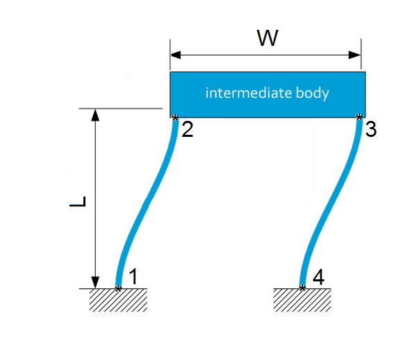
Figure: Parallel flexure guide (from janssenprecisionengineering.com)

To set up the simulation, we need to define the node positions, element connectivity, node properties and the element properties.

We start by defining the positions of the nodes. The origin is located at node 1. Matrix nodes is an n_n×3 matrix for defining the positions of the nodes. Each row represents a node (there are n_n nodes). The row number determines the node number. The first column contains the x-coordinate of the node position, the second column the y-coordinate, and the third column the z-coordinate.

clear   %clear workspace
clc     %clear command window
 
% addpath('spacar') %have this point to the folder where spacar is located
 
%some dimensions
L = 0.1;    %[m]
W = 0.05;   %[m]
 
%% NODE POSITIONS
nodes = [0 0 0;     %node 1
         0 L 0;     %node 2
         W L 0;     %node 3
         W 0 0];    %node 4

Next, the connectivity between nodes needs to be defined. Element connectivity is defined by an n_e×2 matrix. Each row represents an element (there are n_e elements). The row number determines the element number. Each element connects two nodes. The first column contains the number of the node that the element is connected to on one side, the second column the node number that the element is connected to on the other side.

%% ELEMENT CONNECTIVITY
elements= [1 2;     %leafspring between node 1 and 2 
           2 3;     %intermediate body between node 2 and 3
           3 4];    %leafspring between node 3 and 4 

A structure array defines node properties, such as boundary conditions, applied loads, and inertia. The usage is nprops(i).field = value; to assign property field with value value to node i. For a full syntax list with all possible inputs, see SPACAR Light syntax.

First of all, nodes 1 and 4 are fixed:

%% NODE PROPERTIES
nprops(1).fix = true;       %fix node 1
nprops(4).fix = true;       %fix node 4

Furthermore, we would like the parallel flexure guide to start 10 mm deflected to the left and then have it move 20 mm to the right. For this purpose, we prescribe the position of node 2 in x-direction:

nprops(2).displ_initial_x =-0.01; %start with node 2 displaced 10 mm to the left
nprops(2).displ_x =         0.02; %displace node 2 20 mm to the right

Lastly, we apply a load of 5 N in z-direction on nodes 2 and 3:

nprops(2).force_initial = [0 0 5]; %initial load of 5N in z-direction on node 2
nprops(3).force_initial = [0 0 5]; %initial load of 5N in z-direction on node 3

Element properties are defined by a structure array for assigning properties to elements, such as dimensions, material constants, flexibility, and visual appearance. Properties are created in sets, such that the same set of properties can be assigned to multiple elements.

The usage is eprops(i).field = value; to assign property field with value value to set i. For a full syntax list with all possible inputs, see SPACAR Light syntax.

The first element property set is assigned to both leafsprings (elements 1 and 3). The material is steel, width is 50 mm and thickness is 0.5 mm. Elements with flexibility in all directions are used, by setting all deformation modes (1 to 6) to be flexible.

%% ELEMENT PROPERTIES
%first element property set
eprops(1).elems = [1 3];        %assing property set 1 to elements 1 and 3
eprops(1).emod = 210e9;         %E-modulus [Pa]
eprops(1).smod = 70e9;          %shear modulus [Pa]
eprops(1).dens = 7800;          %density   [kg/m^3]
eprops(1).dim = [0.05 0.0005];  %cross-sectional dimension (width and thickness, resp.) [m]
eprops(1).cshape = 'rect';      %rectangular cross-sectional shape 
eprops(1).flex = 1:6;           %fully flexible elements, using all deformation modes (1 to 6) 
eprops(1).orien = [0 0 1];      %width-direction of leafspring oriented in z-direction
eprops(1).color = [0.8549    0.8588    0.8667]; %color in RGB values between 0 and 1

The second element property set is assigned to the intermediate body (element 2). The material is aluminium, width is 50 mm and thickness is 50 mm. The element is fully rigid, which is effected by not making any of the deformation modes flexible (i.e. eprops(2).flex is the default empty vector).

%second element property set
eprops(2).elems = [2];          %assing property set 2 to element 2
eprops(2).dens = 2700;          %density   [kg/m^3]
eprops(2).dim = [0.05 0.025];   %cross-sectional dimension (width and thickness, resp.) [m]
eprops(2).cshape = 'rect';      %rectangular cross-sectional shape
eprops(2).orien = [0 0 1];      %width-direction of leafspring oriented in z-direction
eprops(2).color = [0.1686    0.3922    0.6627]; %color in RGB values between 0 and 1

With all input complete, a call to spacarlight() can be used:

 out = spacarlight(nodes,elements,nprops,eprops);

If the model works, spacarlight automatically runs the static simulation and produces a visualization of the results.

Also, simulation results are stored in the MATLAB workspace in the structure out.

example.m

clear
clc
 
% addpath('spacar') %have this point to the folder where spacar is located
 
%some dimensions
L = 0.1;    %[m]
W = 0.05;   %[m]
 
%% NODE POSITIONS
nodes = [0 0 0;     %node 1
         0 L 0;     %node 2
         W L 0;     %node 3
         W 0 0];    %node 4
 
 
%% ELEMENT CONNECTIVITY
elements= [1 2;     %leafspring between node 1 and 2 
           2 3;     %intermediate body
           3 4];    %leafspring between node 3 and 4 
 
 
 %% NODE PROPERTIES
nprops(1).fix = true;       %fix node 1
nprops(4).fix = true;       %fix node 4
 
nprops(2).displ_initial_x =-0.01; %start with node 2 displaced 10 mm to the left
nprops(2).displ_x =         0.02; %displace node 2 20 mm to the right
 
nprops(2).force_initial = [0 0 5]; %initial load of 5N in z-direction on node 2
nprops(3).force_initial = [0 0 5]; %initial load of 5N in z-direction on node 3
 
 
%% ELEMENT PROPERTIES
%first element property set
eprops(1).elems = [1 3];        %assing property set 1 to elements 1 and 3
eprops(1).emod = 210e9;         %E-modulus [Pa]
eprops(1).smod = 70e9;          %shear modulus [Pa]
eprops(1).dens = 7800;          %density   [kg/m^3]
eprops(1).dim = [0.05 0.0005];  %cross-sectional dimension (width and thickness, resp.) [m]
eprops(1).cshape = 'rect';      %rectangular cross-sectional shape 
eprops(1).flex = 1:6;           %flexible deformations: torsion (2) and out-of-plane bending (3,4) 
eprops(1).orien = [0 0 1];      %width-direction of leafspring oriented in z-direction
eprops(1).color = [0.8549    0.8588    0.8667]; %color in rgb values between 0 and 1
 
%second element property set
eprops(2).elems = [2];          %assing property set 2 to element 2
eprops(2).dens = 2700;          %density   [kg/m^3]
eprops(2).dim = [0.05 0.025];   %cross-sectional dimension (width and thickness, resp.) [m]
eprops(2).cshape = 'rect';      %rectangular cross-sectional shape
eprops(2).orien = [0 0 1];      %width-direction of leafspring oriented in z-direction
eprops(2).color = [0.1686    0.3922    0.6627]; %color in rgb values between 0 and 1
 
 
%% DO SIMULATION
out = spacarlight(nodes,elements,nprops,eprops);