Table of Contents
SPACAR Light FAQ
1. Number of beams per flexible element
For accurate results, it may be necessary to model flexible elements using more than one beam. Whether multiple beams are needed depends on the particular load case and the deformations involved.
Additional beams bring additional degrees of freedom, so that e.g.
- more complex mode shapes can be modelled,
- the deflected shape (in particular for large deformations) can be modelled more accurately,
- a more accurate stress distribution can be obtained.
This means that there’s no general answer to the number of beams that are needed per element. The approach to deciding on the number is to investigate if the quantity of interest (displacement, eigenfrequency, stress, stiffness, etc.) changes with an increasing number of beams. By increasing the number of beams until the quantity of interest doesn’t change anymore, it’s likely that the solution has converged.
The number of beams that are used per element can be set using the eprops(i).nbeams field. See the full syntax list.
For an entirely rigid element, there is no benefit to using more than one beam.
Specifics for the ME module 8 mechatronics project
- For motion in the DOF (the actuation direction of the mechanism), it is likely that the deformation, stiffness, stress and eigenfrequency can be predicted sufficiently accurately with a single beam per flexible element. (You can investigate this using the approach described above.)
- For higher mode shapes, associated with motion in a constrained direction of the mechanism, it is likely that multiple beams are needed per flexible element. A good starting point would be to use
eprops(i).nbeams = 3and investigate if this is enough (i.e. check if the eigenfrequency of interest doesn’t change when further increasing the number). - By default, Spavisual only shows the first 10 mode shapes of the mechanism. To increase this number, see the use of the
opt.customvisfield in the full syntax list. - Increasing the number of beams leads to more degrees of freedom and more eigenmodes (with generally higher eigenfrequencies). The state space and transfer function representations will contain many states. If possible, avoid unnecessary conversions from state space to transfer functions.
- To use such a detailed model in Simulink, pre-process the state space representation to discard eigenfrequencies higher than the Nyquist frequency. See the project lectures for details.
- Add some modal damping (a relative damping of 0.001 to 0.01 for steel materials) to the modes for more representative Bode plots. See the use of the
opt.transferfield in the full syntax list.
2. Overconstraints could not be solved automatically
It is most likely that this error occurs because the model contains loops of elements that are completely rigid. See the figure below for an example.
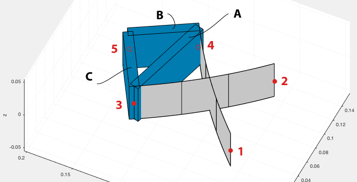
Here, we tried extending the frame by adding a fifth node and two extra rigid elements (B and C). We did this so that we can attach some mass and apply a force on node 5. When running the model, an error now occurs: “Overconstraints could not be solved automatically; partial release information is provided in the output”.
The program is unable to deal with the loop that is created by the rigid elements A, B, and C. With flexible elements, it’s fine to create loops — it’s only rigid loops that should be avoided.
Solution
Remove one of the elements that make up the rigid loop. In the case of this example, we could remove either element B or C — and it would not change the model! Element A still provides the rigid connection between the leaf springs, and we only need B or C to extend the frame towards node 5 in a rigid manner. Visually, it may look a bit different, but structurally, the model is the same. Note that if you’re specifying a density for these rigid elements, the elements also contribute some mass and inertia, so, then, leaving out an element would change the model. In our example, we chose to have rigid elements with zero density (so, massless); we’re placing the relevant mass of the frame in node 5 (using node properties) instead.
Notes
Ground loop: In this example we created a loop using three rigid elements. Note that the fixed world could also be a part of the loop. For instance, modeling just a single rigid element with both nodes fixed would lead to the same error.
Automatic detection: If you’re running MATLAB R2021a (or higher), an extra feature will be available that tries to detect if rigid loops are present. If detected, the nodes involved in this loop will be listed, so that it should be easier to identify the loop.
Manual releases: An alternative solution is to provide appropriate releases for the deformations in the opt.rls field. This way, you can have loops of rigid elements. A future article may detail how to do that exactly …
3. Changing units
When the system parameters are expressed with very small numbers, you may receive the warning “Mass coefficients turn out to be very small” or the related error “Singular mass matrix”. Changing the units of the parameters involving the length dimension may help.
The example file that comes with SPACAR Light assumes meters as the default unit for length. To change to other units, your script should be adjusted in several places, depending on how each physical quantity scales with the length L:
- coordinates of the nodes (
nodes): default unit is m so the coordinates scale as L. - input displacements (
nprops(i).displ_*,nprops(i).displ_initial_*): default unit is m so the displacements scale as L. - (rotations in radians are independent of length)
- moment of inertia (
nprops(i).mominertia): default unit is kg*m^2, so moment of inertia scales as L^2. - forces (
nprops(i).force,nprops(i).force_initial): default unit is N = kg*m/s^2 so force scales as L. - moments (
nprops(i).moment,nprops(i).moment_initial): default unit is N*m = kg*m^2/s^2 so moment scales as L^2. - material stiffness properties (
eprops(i).emod,eprops(i).smod): default unit is Pa = N/m^2 = kg/(m*s^2) so these scale as 1/L. - material density (
eprops(i).dens): default unit is kg/m^3 so density scales as 1/L^3. - cross-sectional dimensions (
eprops(i).dim): default unit is m so these dimensions scale as L. - gravitational acceleration (
opt.gravity): default unit is m/s^2 so acceleration scales as L.
In other words, if your script assumes meters as the unit for length, and you want to go to millimeters, the nodes matrix should be multiplied by 10^3. Likewise, the forces should be multiplied by 10^3, the moments by 10^6, the elasticity and shear modulus by 10^(-3), and all other quantities according to the list above.
Note that output values, so numbers you see in the out structure and in Spavisual, are affected similarly.
4. Bode plots
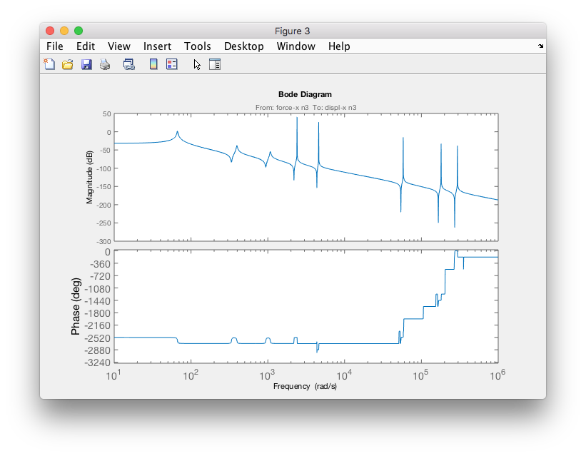
When making Bode plots of the system, in particular with a lot degrees of freedom (e.g. when eprops(i).nbeams is greater than 1), the default phase plot after doing bode(out.statespace) can be hard to interpret:
It can be helpful to go to Properties (after right-clicking) and the Options tab, and:
- uncheck “Wrap phase”
- check “Adjust phase offsets” (the default numbers are generally fine)
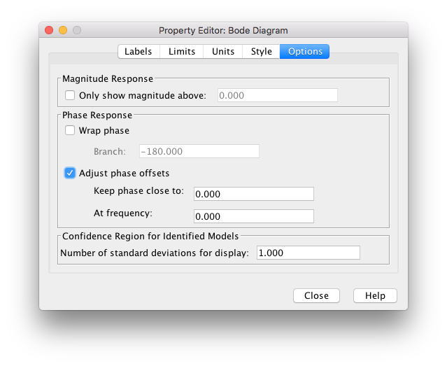
This way, multiples of 360 degrees are subtracted from the phase such that the phase at zero frequency is closest to 0 degrees. After zooming in on the phase:
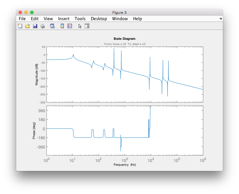
Also see the example on producing transfer functions for tips on making Bode plots that look nicer.
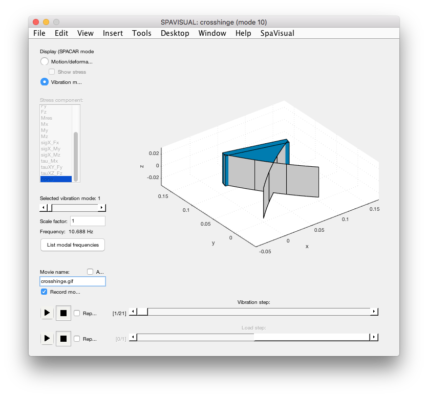
5. Animated GIFs of mode shapes
For presentation purposes, it can be helpful to create an animated GIF of a visualization in Spavisual. You can make a GIF for a particular mode shape or for the general motion of the system. In the Spavisual window, deselect the 'Auto' checkbox for 'Movie name' in the left bottom corner. Select the 'Record movie' checkbox and enter a filename with the extension '.gif'. Then, after clicking the play button for the relevant slider, the animated GIF will be created in the current folder.
Depending on the purpose, you may want to change the appearance of the Spavisual axis in which the model is animated. Sometimes, it could be nice to disable the grid lines or disable the coordinate frame altogether. To do so, add some of the following lines:
% ... model definition ...

out = spacarlight(nodes, elements, nprops, eprops, opt);
ah = out.fighandle.Children(1); %get the handle of the Spavisual axis
axis(ah,'off'); %disable axis (the background in the GIF should become transparent!)
%grid(ah,'off'); %disable just the grid lines