This example shows the computation of the transfer function from input actuator force to output sensor displacement of a parallel flexure guide.

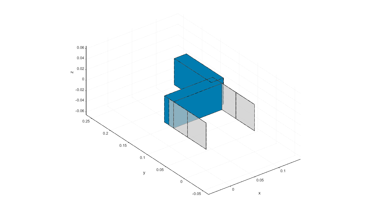
The state-space equations (from which the transfer function follows) can be computed by specifying the desired inputs and outputs of the system. For this example, the actuation force in x-direction on node 3 (a node on the end-effector) is used as the input. Two desired outputs are specified: the first is the displacement in x-direction of node 5, which is where the sensor is located. The second output is the velocity in x-direction at the actuator node; this second output is useful for modeling the back-emf of the actuator.

These inputs and outputs can be specified with the nprops(i).transfer_in and nprops(i).transfer_out arguments. Furthermore, to enable the computation of the state-space equations, the optional field opt.transfer has to be set to true. For details, see the SPACAR Light full syntax. For this case, the MATLAB file that defines the flexure mechanism is supplemented with

nprops(3).transfer_in  = {'force_x'};       %Input 1 for state-space equations
nprops(5).transfer_out = {'displ_x'};       %Output 1 for state-space equations
nprops(3).transfer_out = {'veloc_x'};       %Output 2 for state-space equations
...
opt.transfer = {true 0.01};       %Calculation of state-space equations (with relative damping 0.01)

Note that

• the state-space equations can only be computed for an undeformed flexure mechanism. Therefore, no external loads (actuation force) or input displacements are allowed when computing state-space equations. (An error message will appear if you do specify this.)
• velocity outputs are supported as well;
• relative damping for all modes of the system can be specified optionally by means of the opt.transfer field.

For details, see the SPACAR Light full syntax.

The resulting transfer function between the input and the first output is plotted in the figure below. The first eigenfrequency is approximately 10 rad/s; the first parasitic eigenfrequency appears at 360 rad/s.

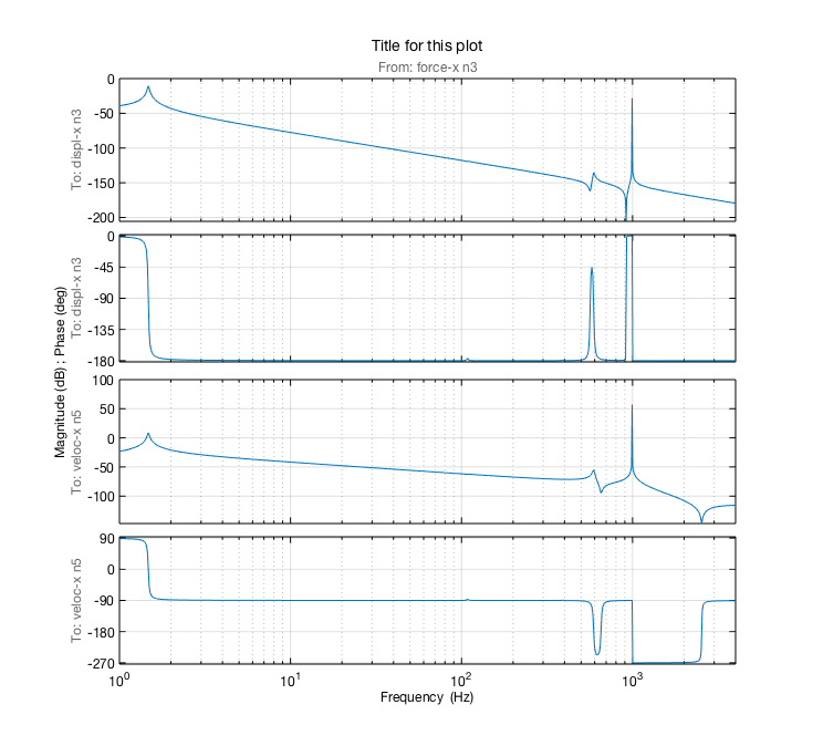
Note that in case of multiple inputs and/or outputs, the resulting state-space structure in MATLAB will also indicate with named labels what these inputs and outputs are (i.e. node number and displacement, velocity or force).

An example file for providing the input for SPACAR Light and plotting the transfer function is provided below.

example.m

% EXAMPLE SCRIPT FOR RUNNING SPACAR LIGHT
% This example simulates a parallel flexure guide and computes the transfer
% function from actuator force to sensor displacement
clear
clc
 
%% NODE POSITIONS
%           x y z
nodes = [   0 0 0;      %node 1  
            0 0.1 0;    %node 2  
            0.1 0.1 0;  %node 3
            0.1 0 0;    %node 4
            0.1 0.2 0]; %node 5 
 
 
%% ELEMENT CONNECTIVITY
%               p   q
elements = [    1   2;  %element 1
                2   3;  %element 2
                3   4;  %element 3
                3   5]; %element 4
 
 
%% NODE PROPERTIES  
%node 1
nprops(1).fix               = true;         %Fix node 1
 
%node 3
nprops(3).transfer_in  = {'force_x'};       %Input for state-space equations
nprops(5).transfer_out = {'displ_x'};       %Output nr 1 (displ. in x-direction on node 5) for state-space equations
nprops(3).transfer_out = {'veloc_x'};       %Output nr 2 (veloc. in x-direction on node 3) for state-space equations
 
%node 4
nprops(4).fix               = true;         %Fix node 4
 
 
%% ELEMENT PROPERTIES
%Property set 1
eprops(1).elems    = [1 3];            %Add this set of properties to elements 1 and 3
eprops(1).emod     = 210e9;            %E-modulus [Pa]
eprops(1).smod     = 70e9;             %Shear modulus [Pa]
eprops(1).dens     = 7800;             %Density [kg/m^3]
eprops(1).cshape   = 'rect';           %Rectangular cross-section
eprops(1).dim      = [50e-3 0.2e-3];   %Width: 50 mm, thickness: 0.2 mm
eprops(1).orien    = [0 0 1];          %Orientation of the cross-section as a vector pointing along "width-direction"
eprops(1).nbeams   = 2;                %2 beam elements for simulating these flexures
eprops(1).flex     = 1:6;              %Fully flexible beam
eprops(1).color    = 'grey';           %Color of elements
eprops(1).opacity  = 0.7;              %Opacity of elements
% eprops(1).warping  = true;             %Enable modeling of warping, e.g. for the effect of constrained warping
 
%Property set 2
eprops(2).elems    = [2 4];            %Add this set of properties to element 2 and 4
eprops(2).dens     = 7800;             %Density [kg/m^3]
eprops(2).cshape   = 'rect';           %Rectangular cross-section
eprops(2).dim      = [50e-3 25e-3];    %Width: 50 mm, thickness: 25 mm
eprops(2).orien    = [0 0 1];          %Orientation of the cross-section as a vector pointing along "width-direction"
eprops(2).nbeams   = 1;                %1 beam element for simulating this component
eprops(2).color    = 'darkblue';       %Color of elements
 
 
%% OPTIONAL ARGUMENTS
opt.transfer = {true 0.01};       %Calculation of state-space equations (with relative damping 0.01)
opt.filename = 'file';            %Names of files that are produced
 
%% CALL SPACAR_LIGHT
out = spacarlight(nodes, elements, nprops, eprops, opt);
 
%% Plot transfer function
%set some convenient defaults for the plot. Not necessary, but they can improve the plots
bodeopt = bodeoptions;
bodeopt.Title.String = 'Title for this plot';
bodeopt.FreqUnits = 'Hz'; %default frequency units
bodeopt.Xlim = [1,4000]; %frequency axis limits
bodeopt.Grid = 'on'; %show a grid
 
bodeopt.Title.FontSize = 14; %font size for title
bodeopt.XLabel.FontSize = 12; %font size for xlabels
bodeopt.YLabel.FontSize = 12; %font size for ylabels
bodeopt.TickLabel.FontSize = 12; %font size for the ticks (numbers on axes)
bodeopt.InputLabels.FontSize = 12;
bodeopt.OutputLabels.FontSize = 12;
 
bodeopt.PhaseMatching = 'on'; %phase matching: adding multiples of 360 so that:
bodeopt.PhaseMatchingFreq = 1; %--at this frequency
bodeopt.PhaseMatchingValue = 0; %--the phase is close to this value
 
h = bodeplot(out.statespace,bodeopt); %make the plot