This is an old revision of the document!
SPACAR Light
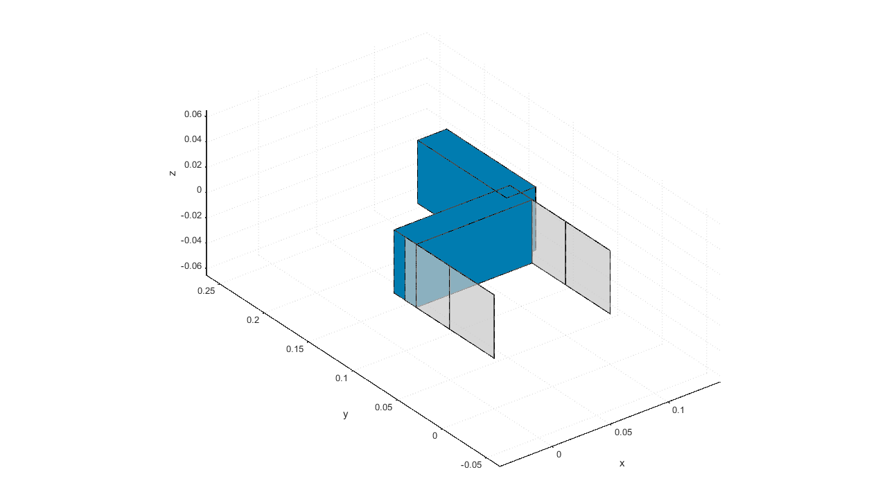
Example: Compute transfer function of a parallel flexure guide
This example shows the computation of the transfer function from actuator force (force in x-direction on the end-effector) to stage displacement (motion in x-direction of the end-effector) of a parallel flexure guide.
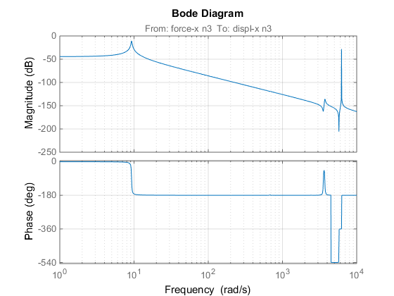
The transfer function (state-space equations) can be computed by specifying the input and output for the transfer function. For this example, actuation force in x-direction on node 3 (a node on the end-effector) is used for input, and displacement in x-direction of node 3 is used for the output. This can be specified with the nprops(i).transfer_in and nprops(i).transfer_out arguments. Furthermore, for computation of the state-space equations, the optional argument opt.transfer is required. For this specific case this results in:
nprops(3).transfer_in  = {'force_x'};       %Input for state-space equations
nprops(3).transfer_out = {'displ_x'};       %Output for state-space equations{'displ_x'};
...
opt.transfer = {true 0.01};       %Calculation of state-space equations (with relative damping 0.01)
It has to be noted that the state-state equations can only be computed for an undeformed flexure mechanism. Therefore, no external loads (actuation force) or input displacements are allowed when computing state-space equations.
The resulting transfer function is plotted in the figure below.
An example file for providing the input for SPACAR Light is provided below.
- example.m
% EXAMPLE SCRIPT FOR RUNNING SPACAR LIGHT
% This example simulates a parallel flexure guide and computes the transfer
% function from actuator force to sensor displacement
clear
clc

%% NODE POSITIONS
%           x y z
nodes = [   0 0 0;      %node 1
            0 0.1 0;    %node 2
            0.1 0.1 0;  %node 3
            0.1 0 0;    %node 4
            0.1 0.2 0]; %node 5


%% ELEMENT CONNECTIVITY
%               p   q
elements = [    1   2;  %element 1
                2   3;  %element 2
                3   4;  %element 3
                3   5]; %element 4


%% NODE PROPERTIES
%node 1
nprops(1).fix               = true;         %Fix node 1

%node 3
nprops(3).transfer_in  = {'force_x'};
nprops(3).transfer_out = {'displ_x'};

%node 4
nprops(4).fix               = true;         %Fix node 4


%% ELEMENT PROPERTIES
%Property set 1
eprops(1).elems    = [1 3];            %Add this set of properties to elements 1 and 3
eprops(1).emod     = 210e9;            %E-modulus [Pa]
eprops(1).smod     = 70e9;             %G-modulus [Pa]
eprops(1).dens     = 7800;             %Density [kg/m^3]
eprops(1).cshape   = 'rect';           %Rectangular cross-section
eprops(1).dim      = [50e-3 0.2e-3];   %Width: 50 mm, thickness: 0.2 mm
eprops(1).orien    = [0 0 1];          %Orientation of the cross-section as a vector pointing along "width-direction"
eprops(1).nbeams   = 2;                %4 beam elements for simulating these elements
eprops(1).flex     = 1:6;        	   %Model out-of-plane bending (modes 3 and 4) as flexible
eprops(1).color    = 'grey';
eprops(1).opacity  = 0.7;
eprops(1).cw       = true;

%Property set 2
eprops(2).elems    = [2 4];            %Add this set of properties to element 2
eprops(2).dens     = 7800;             %Density [kg/m^3]
eprops(2).cshape   = 'rect';           %Rectangular cross-section
eprops(2).dim      = [50e-3 25e-3];    %Width: 50 mm, thickness: 10 mm
eprops(2).orien    = [0 0 1];          %Orientation of the cross-section as a vector pointing along "width-direction"
eprops(2).nbeams   = 1;                %1 beam element for simulating this element
eprops(2).color    = 'darkblue';


%% OPTIONAL ARGUMENTS
opt.transfer = {true 0.01};       %Calculation of state-space equations (with relative damping 0.01)

%% CALL SPACAR_LIGHT
out = spacarlight(nodes, elements, nprops, eprops, opt);

%% Plot transfer function
figure
bode(out.statespace,{1,10000})
grid minor